It is known that cluster analysis is one of the directions of data analysis, which studies the methods of dividing the set of source data into separate classes (clusters) using some proximity functions [1]. In this case, the data elements are grouped into clusters according to the principle of maximizing intracluster and minimizing intercluster communications. Formed clusters can later be used to classify newly arriving data and create templates for data processing (since data elements belonging to the same cluster have similar properties determined by selected proximity functions).
Let's look at the most well-known methods of cluster analysis. Perhaps the most common is the k-means method [2], aimed at minimizing the total quadratic deviations of cluster points from their centers. The main disadvantage of this method is the need to know in advance the number of clusters. One of the variations of the k-means method is the k-median method, in which its median is taken as the center of a cluster. EM-algorithm (Expectation-Maximization) is used when the data are described using a model with hidden variables [3]. The EM algorithm works iteratively, each iteration consists of two steps: E calculating the expected values of hidden variables, M maximizing the likelihood function, which updates the probabilities of data elements belonging to specific clusters. Algorithms of the FOREL family are aimed at separating objects into separate clusters that are in areas of maximum concentration [4]. These algorithms are rarely used, since they require some a priori knowledge about the data being analyzed, and the result of their work strongly depends on the initially selected cluster search points. You can also note the use of Kohonen artificial neural network for clustering, or a self-organizing feature map [5]. Kohonen's neural network contains two layers, the neurons of the output layer correspond to clusters, which produce the larger signal, the closer the data element to the network is located from the corresponding cluster. By changing the size of the output layer, you can achieve a more detailed clustering of data. Genetic algorithms based on a combinatorial search for a solution by applying natural evolution mechanisms (inheritance, mutation, selection, crossing-over) to instances of dividing a set of data into clusters are also used for clustering data [6]. Finally, we should note hierarchical algorithms that allow to build data combining trees into clusters by successively merging small clusters into larger ones, until the entire set of data is divided into the required number of clusters [7].
From the methods for detecting outliers, four main directions can be emphasized. They use different characteristics, on the basis of which decisions on the recognition of an object as an outlier are made: data on statistical distribution (distribution-based), distance between elements (distance-based), local data density (density-based), cluster deviation (deviation-based) [8]. Statistical methods for determining outliers are used mainly for one-dimensional data, when the hypothesis of the conformity of data elements to a certain distribution is checked using a priori or accumulated information on the distribution [9]. Among the numerous criteria for statistical determination of outliers, we can mention the criteria of Chauvene, Irwin, Grubbs and many others. As a method for determining outliers using the distances between elements, we can note the method of k nearest neighbors [10]. In this classification method, a new data element refers to the cluster to which most of its already classified neighbors belong. The criterion for the release in this case is the absence of the mentioned majority, which makes it impossible to make a choice. The method of determining the local density involves calculating the density of data at each point in the data set and recognizing the outlier of a data element whose density differs significantly from the density of its neighborhood [11]. Finally, the latter direction involves the clustering of data, after which some statistics are collected within each cluster. Those data elements whose characteristics are very different from the statistical characteristics of their cluster are recognized as outliers.
The article discusses the method of determining outliers, based on the implementation of hierarchical data clustering and subsequent analysis of the constructed cluster merge tree.
Description of the hierarchical clustering method using dendrogram construction
This section describes the method of hierarchical or sequential clustering of data represented by points in k-dimensional space. The initial data of the hierarchical clustering algorithm are a set of n points P = {P1, P2, … , Pn}, and the number of clusters m ≤ n, into which the given set of points should be divided. At the beginning of the algorithm, we consider the reduced set of points as a set of clusters Q1 = { P1}, Q2 = {P2}, …, Qn = {Pn}. While the current number of clusters exceeds the specified number m, we perform the sequential merging of clusters into larger ones. At each step, we will merge only the two nearest clusters. Let in the considered set of clusters Q1, Q 2, … ,Qt the closest in some sense are the clustersQi and Qj (i < j). Then after combining them, the new set of clusters will look like 
The result of clustering strongly depends on the proximity function, which is used to determine a pair of clusters for merging. We will consider the following types of proximity functions [12]. The minimum local distance between clusters will be called the value
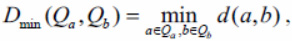
where d(a, b) - arbitrary proximity function between two points a and b. In the following, we will also call this function the distance, although in the general case it may not be a distance. Similarly, we introduce two more proximity functions for a pair of clusters. The maximum local distance between clusters is called 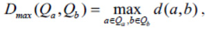
and the average distance between clusters is
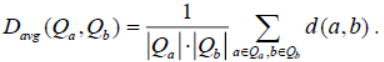
Now consider the functions that will be used as the distance between individual points. First, we use
lp - norm, which is given by the formula

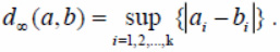
and gives the Euclidian distance in case p = 2 and the sum of the modules of the differences of the corresponding coordinates in the case p = 1. When the value of p goes to infinity, we get a supremum norm written in the form
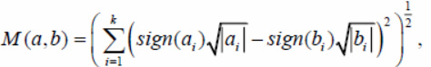
In addition to the considered distance functions, we will also consider the Jeffreys – Matusita measure corrected for the region of negative coordinate values, as shown in the formula
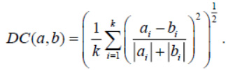
also a measure known as the divergence coefficient, similarly corrected for a region of negative coordinate values
So, we fix a specific view of the distance function between clusters and perform hierarchical clustering
for this function. In the process of performing the clustering procedure, we build a dendrogram – clustering
tree [13]. To build a dendrogram, each cluster will be assigned a binary tree (Fig. 1).
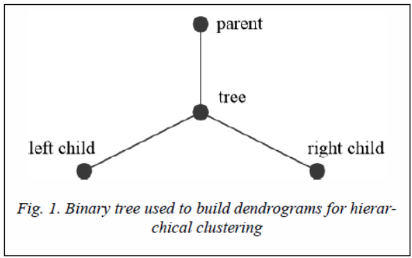
A tree can have only two descendants (binary trees corresponding to the clusters from which the current cluster was obtained), as well as one parent (a binary tree corresponding to the cluster in which the current cluster enters as part), as shown in Figure 1. Before the clustering begins each point of the considered set obtains its own tree without descendants and parents. The tree accumulates a specific point. At each step of combining two clusters, the corresponding trees become descendants of the newly created tree. The process continues until exactly m trees remain, each of which corresponds to a separate cluster. The clustering process can be continued until all the trees are combined into one tree, which is the complete dendrogram of hierarchical clustering.
Consider as an example two simple clustering dendrograms composed for two test sets of points using a simple Euclidean distance between points and an average distance to determine the proximity of two clusters. First consider the set of points P = {(x,x)|x= 1, 2, …, 16}. It's just a set of 16 points lying on a line y=x. When clustering is performed, first 8 pairs of points will be merged, where the distance between the points in each pair is equal to  , after which we get 8 clusters whose centers are also located on a straight line y=x at regular intervals. Then they will be combined in pairs into 4 larger clusters, then in 2, and in the end there will be one cluster. The result of clustering is shown in Figure 2.
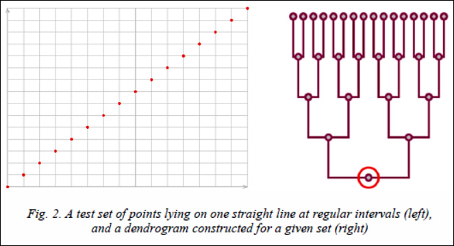
The figure shows that the set of points does not contain outliers, the dendrogram built during clustering is a balanced tree.
Now consider another set of points whose coordinates are given by the formula P = {(x, 2x)| x = 1, …, 8}.
This set of points lies on the graph of the exponent. In the first clustering step, the first two points will merge into a larger cluster. At each next step, the next point on the graph will be added to the already existing cluster, since the distance between it and the cluster is less than the distance between any two free points. As a result, a completely unbalanced dendrogram can be observed (Fig. 3). In this case, when setting a goal to find outliers from the proposed data set, a decision should be made to exclude a point that joined the cluster later than the others. We define more clearly the characteristic with which we will identify outliers.
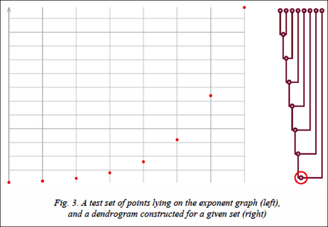
Suppose that for some data set a complete dendrogram is constructed before all points are merged into one cluster. This dendrogram contains information about all intermediate clusters that were formed during the clustering process. For each node of the dendrogram t, it is possible to naturally determine the height function h(t). For leaf nodes this function is equal to one, and for nodes with descendants it is one more than the maximum of the heights of its two descendants. The fact of late attachment of a certain data element to an already formed cluster means that two trees merge together with a large difference between the values of their heights. That is the value h(p(t)) – h( t) is great, where p(t) – parent of t. There is one inaccuracy in this formula. If the tree t in itself is an already formed cluster, then you should not rush to recognize it as an outlier, even if merging with another cluster does not happen soon. To take this into account, the final value should be divided by the width of the tree, or the number of leaf vertices contained in it (we denote this value by w(t)). Thus, we obtain the final outlier identifier, determined using the formula
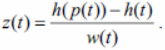
We assume that all nodes of the dendrogram with the largest value of the function z are outliers.
Applying a voting method to determine the most likely outliers
The method discussed in the previous section allows you to identify potential outliers from a dataset when building a hierarchical clustering dendrogram. However, as already noted, the type of dendrogram substantially depends on the choice of the distance function between points and the proximity function between clusters. And if dendrograms are different, then candidates for outliers will be different. To resolve this dispute, apply a voting method to determine outliers. That is, we will perform clustering for all the available distance functions between points, and for each distance function use all the proximity functions between the clusters. For each fixed mode, we will determine a constant number of potential outliers, and then for each leaf node marked as a potential outlier, increment its counter. After all possible clustering modes have been performed, outliers are recognized as those data elements whose outlier counters are maximum.
Analysis of the results
To test the proposed voting method for determining outliers during hierarchical clustering, test sets of 200 two-dimensional points were generated in the square –50.0 ≤ ≤x≤ 50.0, –50.0 ≤y≤ 50.0 (Fig. 4), clustering on 12 clusters was performed for each set. The minimum local distance (min), the maximum local distance (max), and the average distance (avg) were used as the proximity functions between the clusters. As functions of distance between points the following functions were used: d1 ((the sum of the modules of the differences of the corresponding coordinates), d2 (Euclidean distance), d4 ((distance using the norm l4), d ∞(supremum-norm), M (measure of Jeffreys-Matusita), DC (divergence coefficient). Thus, there are a total of 18 clustering execution modes.
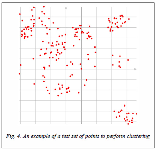
Figure 5 illustrates the visualization of a hierarchical clustering tree. The top row of leaf nodes corresponds to the original array of clustered points. Each cluster as data encapsulates a point on the plane, which is its center. For leaf nodes, this is just the starting point. When two clusters merge, which correspond to the trees t1 andt2 with the centers p1 and p2, respectively, a new cluster t is formed with the center at the point
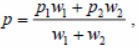
where w1 and w2 are the width of trees t1 and t2, respectively. The nodes corresponding to the desired clusters in Figure 5 are circled in concentric circles. The figure also shows 3 outliers.
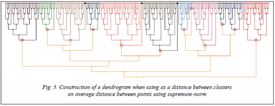
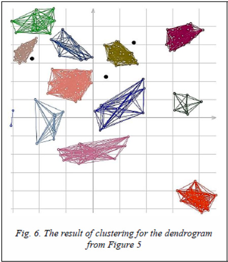
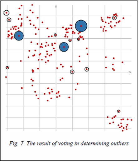
Figure 6 shows the visualization of dividing points into clusters with outliers, and figure 7 shows three outliers defined by voting methods after clustering by all 18 modes (the radius of the outlier label is proportional to the number of votes cast for this point).
After a vote on the determination of outliers, the question arises: which functions of the distances between clusters are most appropriate in identifying clusters. To determine this, experiments were conducted with 10 different sets of test data, the results of which are presented in a matrix (Fig. 8).

In Figure 8, all used clusterings are shown vertically (all variants of cluster proximity functions), 10 test cases are marked horizontally. Each cell of the matrix contains a number from 0 to 3, corresponding to the number of guessed outliers in a particular clustering mode. For the analysis of the matrix, at first, the set with the lowest average guessing index (set No. 9) and the set with the highest average guessing index (set No. 4) were excluded from the analysis. It was further noted that the use of the minimum local distance during clustering leads to a decrease in the number of guessed outliers, therefore, these modes were also removed. As can be seen from the figure, the greatest number of guessing is achieved using the distance functions d4, d2 and d 1 in descending order.
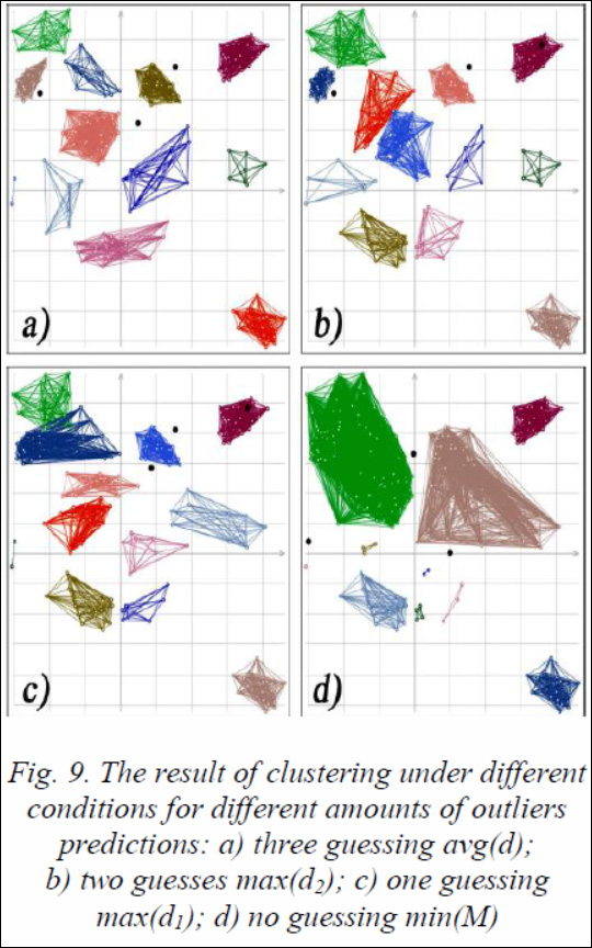
At the end of the experiment, Figure 9 shows the visualization of the clustering of the test set of points from Figure 7 with different distance functions with different numbers of guessing outliers. From the above visualization, it can be noted that clustering with an outlier guessing value of 2 and 3 looks more adequate than in modes where the number of guesses is 0 or 1.
Conclusion
In the framework of this work, the algorithm of hierarchical clustering of two-dimensional points using various proximity functions between clusters is considered. A voting method was proposed to identify potential candidates for outliers, and an analysis was conducted to identify those proximity functions that achieve the greatest number of outliers predictions. It is noted that clustering performed on such modes visually looks more adequate than on modes with a low number of guesses.
Research conducted within the framework of this work can be continued, since it would be interesting to see how the voting results will change if use not hierarchical clustering methods.
The work was done in JSCC RAS with the support of RFBR grants 18-29-03236 and 19-57-60004.
References
1. Tuffery S. Data mining and statistics for decision making. NY, Wiley, 2011, 704 p.
2. Jain A.K. Data clustering: 50 years beyond K-means. Patt. Recogn. Lett., 2010, vol. 31, no. 8, pp. 651–666.
3. McLachlan G.J., Krishnan T. The EM Algorithm and Extensions. NY, Wiley, 1997, 304 p.
4. Tyurin A.G., Zuyev I.O. Klasternyy analiz, metody i algoritmy klasterizatsii. Vestn. MGTU MIREA, 2014, vol. 2, no. 3. pp. 86–97.
5. Hecht-Nielsen R. Neurocomputing. NY, Addison-Wesley, 1990, 433 p.
6. Segaran T. Programmiruyem kollektivnyy razum [Programming collective intelligence]. Saint-Petersburg, Simvol-Plyus, 2008, 368 p.
7. Pestunov I.A., Rylov S.A., Berikov V.B. Iyerarkhicheskiye algoritmy klasterizatsii dlya segmentatsii mul'tispektral'nykh izobrazheniy. Avtometriya, 2015, vol. 51, no. 4, pp. 12–22.
8. Han J., Kamber M. Data Mining: Concepts and Techniques. Morgan Kaufmann Publ., 2006, 368 p.
9. Buxovecz A.G., Moskalev P.V., Bogatova V.P., Biryuchinskaya T.Y. Statisticheskij analiz dannyh v sisteme R. Voronezh, Izd-vo VGAU, 2014, 124 p.
10. Lantz B. Machine Learning with R. UK, Birmingham-Mumbai, Pack Publ., 2013, 454 p.
11. Breunig M., Kriegel H.-P., Ng R.T., Sander J. LOF: Identifying density-based local outliers. Proc. ACM SIGMOD 2000 Int. Conf. on Management of Data, USA, Dalles, TX, 2000. URL: http://www.dbs.ifi.lmu.de/Publikationen/Papers/LOF.pdf (accessed April 3, 2019).
12. Dyuran B., Odell P. Klasternyj analiz [Cluster analysis]. Мoscow, Statistika, 1977, 128 p.
13. Ye N. Data mining: Theories, algorithms, and examples. USA, Boca Raton, CRC Press., 2014, 329 p.
УДК 004.622
DOI: 10.15827/2311-6749.19.2.4
ОБНАРУЖЕНИЕ ВЫБРОСОВ МЕТОДОМ ГОЛОСОВАНИЯ ПРИ ПРОВЕДЕНИИ ИЕРАРХИЧЕСКОЙ КЛАСТЕРИЗАЦИИ ДАННЫХ
А.А. Рыбаков , к.ф.-м.н., ведущий научный сотрудник, rybakov. aax@ gmail. com, rybakov@ jscc. ru;
С.С. Шумилин , старший инженер, shumilin@ jscc. ru
(Межведомственный суперкомпьютерный центр РАН - филиал НИИСИ РАН,
г. Москва, 119334, Россия)
В настоящее время часто приходится сталкиваться с задачей извлечения полезной информации из большого объема исходных сырых данных. Этот процесс, получивший название Data Mining, объединяет в себе различные подходы к анализу и обработке данных, однако всегда начинается с одного конкретного этапа - очистки данных. Сырые данные, поступающие на вход для анализа, часто оказываются неполными, слабоструктурированными, содержат дублирующую информацию и аномалии. Наличие аномалий в массиве входных данных может привести к неверной трактовке извлекаемой информации, к ошибкам в предсказании и сильно снижает ценность получаемых знаний. Поэтому так актуальна задача разработки новых подходов к устранению аномалий, или выбросов.
В данной статье рассматривается подход к обнаружению выбросов, основанный на иерархической кластеризации данных и применении метода голосования для выявления наиболее вероятных кандидатов на роль выбросов.
Ключевые слова : анализ данных, иерархическая кластеризация, метод голосования, обнаружение выбросов.
Литература
1. Tuffery S. Data mining and statistics for decision making. NY, Wiley, 2011 , 704 p.
2. Jain A.K. Data clustering: 50 years beyond K-means. Patt. Recogn. Lett., 2010, vol. 31, no. 8,
pp. 651–666.
3. McLachlan G.J., Krishnan T. The EM Algorithm and Extensions. NY, Wiley, 1997, 304 p.
4. Тюрин А.Г., Зуев И.О. Кластерный анализ, методы и алгоритмы кластеризации // Вестн. МГТУ МИРЭА. 2014. № 2. Вып. 3. С. 86–97.
5. Hecht-Nielsen R. Neurocomputing. NY, Addison-Wesley, 1990 , 433 p.
6. Сегаран Т. Программируем коллективный разум. СПб: Символ-Плюс, 2008. 368 с.
7. Пестунов И.А., Рылов С.А., Бериков В.Б. Иерархические алгоритмы кластеризации для сегментации мультиспектральных изображений // Автометрия. 2015. Т. 51. № 4. С. 12–22.
8. Han J., Kamber M. Data Mining: Concepts and Techniques. Morgan Kaufmann Publ., 2006 , 368 p.
9. Буховец А.Г., Москалев П.В., Богатова В.П., Бирючинская Т.Я. Статистический анализ данных в системе R. Воронеж: Изд-во ВГАУ, 2014. 124 с.
10. Lantz B. Machine Learning with R. UK, Birmingham-Mumbai, Pack Publ., 2013 , 454 p.
11. Breunig M., Kriegel H.-P., Ng R.T., Sander J. LOF: Identifying density-based local outliers. Proc. ACM SIGMOD 2000 Int. Conf. on Management of Data, USA, Dalles, TX, 2000. URL: http://www.dbs.ifi.lmu.de/Publikationen/Papers/LOF.pdf (дата обращения: 03.04.2019).
12. Дюран Б., Оделл П. Кластерный анализ. М.: Статистика, 1977. 128 с.
13. Ye N. Data mining: Theories, algorithms, and examples. USA, Boca Raton, CRC Press. 2014, 329 p.
Comments