Determining the Location of Players in Virtual Soccer

Currently, artificial intelligence is surging. Some platforms are designed for scientific research in the field of artificial intelligence (for example, Gym OpenAI, GVGAI), others are for competitions (RoboCup 2D Soccer Simulation League Champion [1], RoboCup Rescue Simulation [2]). Simulation in virtual soccer is used for research, development, and comparison of multi-agent systems, to simplify this process, it is possible to use Soccer Simulation [3], which provides the suitable tools.

The environment of virtual soccer is very dynamic and can well simulate the conditions of the real world. In particular, they assumed full autonomy of the player management programs and the provision of visual and audio information to the players with a predetermined error and distance restrictions. Various methods are used to control and position players: using decision trees, which form options for further actions based on the current state (tree node) and input data [4, 5], using random finite sets [4, 6], the Monte Carlo method [4, 7], fuzzy automata [8], probabilistic automata [9], convolutional neural networks [1, 4, 10].

Decision-making can be based only on the current state of the world or on several previous states. At the same time, an agent that considers the previous states will act more efficiently and therefore win against a player who decides to consider only one state. Planning actions based on the change history in the situation is important when creating intelligent agents. Action planning involves predicting changes in the field situation, considering the actions that can be performed in the situation created. The prediction can be carried out based on both incoming data and change, along with updated information at each clock cycle [7], and the formed model with its gradual refinement [11]. We consider information about visible objects in both cases, but for objects that were recently in vision and then disappeared from it, the behavior is unknown. Considering their behavior will significantly enrich the model and improve the accuracy of predicting the development of the situation in the field.

We should note that in the conditions of virtual soccer, the coordinates of the player are also unknown – we calculate them based on the visible flags placed around and on the playing field. This problem is not always solved unambiguously since the information is provided to the control program with some error [12].

Problems' Solutions

The virtual soccer platform provides noise for the data arriving to players from the visual sensor, which imposes restrictions on how to solve the problem. We can apply the algorithms specified below.

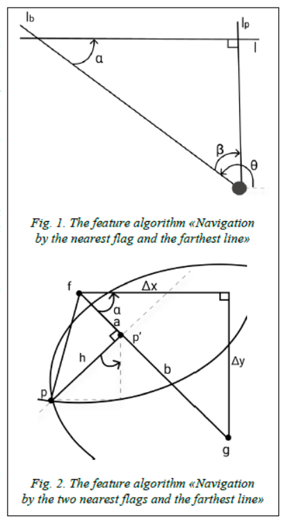
1. Navigate by the nearest flag and the farthest line.

Calculations are performed based on the trigonometric formulas-the static point in the field closest to the agent is selected (the midfield, the team's goal, the four areas in front of the goal, to the right and left of them, the area directly in front of the goal) and the far visible line of the field boundary (Fig. 1). Using the angle calculated by the formula: β = –sin(α)(90 –|α|), where α – the angle at which the line is visible, and the available absolute coordinates of the flag, the agent calculates its real coordinates [13]:

(px, py) = (fx, fy) – π(fr,fφ + (90 + β)), where fx, fy, fr, fφ – the x and y coordinates of the flag, as well as the distance to it and the angle at which the flag is visible, respectively; π is the function of converting polar coordinates to Cartesian coordinates.:

π(r, φ) = (rcos(φ), rsin(φ)).

2. Navigate by the two nearest flags and the farthest line.

Calculations for this method are based on trigonometric formulas using the two static points closest to the agent in the field (the midfield, the team goal, the four areas in front of the goal, to the right and left of them, the area directly in front of the goal) and the far line (Fig. 2). The distance to the flag and its coordinates define a circle of possible positions, and the intersection of the two circles determines the
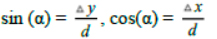
player's position. The distance between flags (f, g):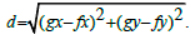

Calculating the player absolute coordinates [13]:

(px, py) = (px’ – h sign sin(α), py’+ h sign cos(α)),

where (px’, py’) = (fx + a cos (α), fy + a sin (α)),

3. Navigation using the particle filter.

The particle filter is a method for determining the absolute coordinates of a player, according to which a set of hypotheses about their current values is created to estimate the coordinates. The algorithm for determining the absolute coordinates based on the particle filter includes the following steps.

Step 1. Initialization-getting information about the first step of the work, while generating hypotheses randomly.

Step 2. Prediction-guess the player's location based on the information received from the server.

Step 3. Correction-calculation of the weight coefficients, and before this calculation, the particles are filtered out by calculating the upper and lower bounds of the hypotheses (particles that are not included in the range are removed) and re-sampling – removing hypotheses with low weight and duplicating hypotheses with high weight.

Step 4. State estimation-calculation of absolute coordinates as the weighted sum of all particles' states [13, 14].

4. Navigation using the Kalman filter.

The method allows you to get an estimate of the object's state vector (in this case, the player's coordinates) based on a series of noisy measurements. It implemented the solution in several steps.

Step 1. Post-information analysis received from the visual sensor (information from the server). If you have saved data, you can skip the parsing step and focus on the analysis.

Step 2. Cyclic processing of all possible pairs-iterating over all pairs of visible flags and calculating the absolute coordinates from these flags.

Step 3. Calculation of the sensor error variance – the primary stage at which the quality of this method is determined: 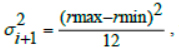, where rmax and rmin are the maximum and minimum possible distance values; is the error dispersion.

Step 4. Update the value of the Kalman gain (K), considering the resulting dispersion. The coefficient value must provide the maximum proximity of the calculated optimal values of the absolute coordinates to their true values: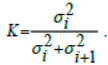

Step 5. Correction using the Kalman coefficient of the estimated value of the absolute coordinates of the agent in this iteration:x_i₊₁= x_i*K+(1 –K)*(x_i+ Δx), y_i₊₁= y_i*K+(1– K)*(y_i+ Δy), where Δx, Δy is the expected change in coordinates.

Thus, the real coordinates of the player are calculated [13–15].

5. Monte Carlo method and Data aggregation.

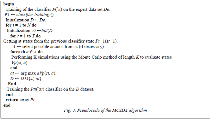
The method is based on a combination of Monte Carlo search and data aggregation (MCSDA) [7] to adapt the agent's actions to the opposing team's game strategies. Using a simple domain representation, the algorithm is trained in a controlled way on an initial data set comprising several simulations of actual games, similar to [16]. The method allows you to control navigation and helps in deciding in the field. The algorithm uses a set of state-action pairs as input. Then the classifier ^π is trained, and at each iteration, the algorithm expands its data set ~π by generating the state st at each time step, with the expected value maximized by the function V_p (s_t, a). After the entire cycle, the aggregated data set is used to train a new classifier ~π (Fig. 3).

1. Random finite sets method

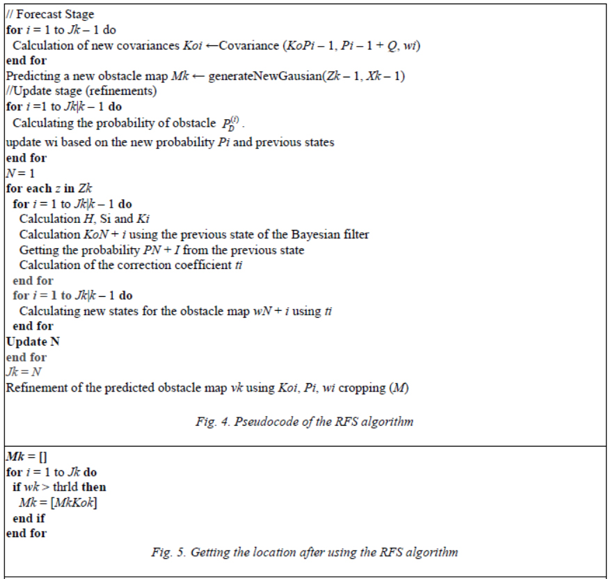
The method provides the map construction of robot movements using random finite sets (RFS) [6]. It is applied to the assessment problem of the teammate and opponent position in the SPL League and comprises two steps.

Step 1. Prediction-creating hypotheses about the appearance of new obstacles for the next cycle of work.

Step 2. Update-calculation of the discoverability of new obstacles at a given point, after which there are the operations of pruning and merging elements (Gaussians that are determined close enough, through the Mahalanobis distance threshold, are combined into one).

Figure 4 shows the pseudocode of the algorithm.

This algorithm is used to calculate obstacle maps in visible space. To get the position of an object in the field, you need to estimate the weight of each element. The mean vector sets if and added to the vector representing the current map (Figure 5).

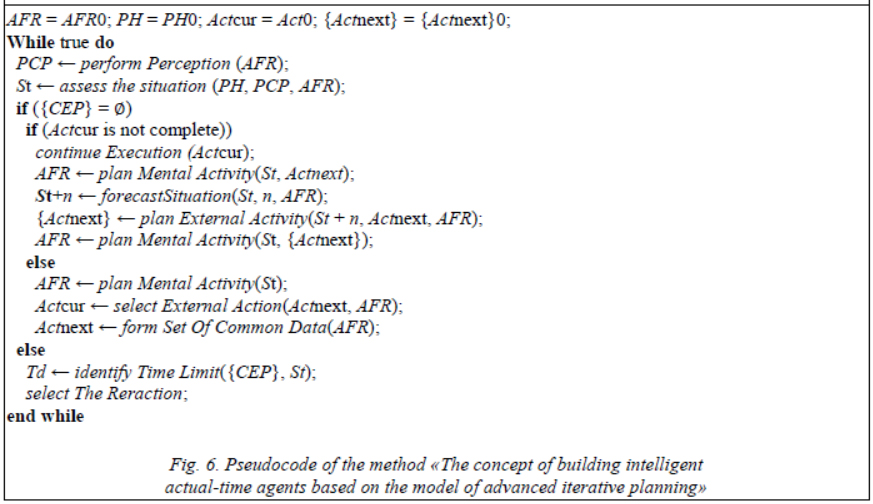
2. The concept of constructing the intelligent real-time agents based on the model of advanced iterative planning.

For decision-making by players, the concept of constructing a model of advanced iterative planning is used [10]. The steps are generalized since because of the exponential growth of the trees of possible events, accurate prediction is not possible. The calculation cycle includes the following steps.

Step 1. Getting sensory information from the perception subsystem.

Step 2. Assess the situation.

Step 3. Predicting the situation.

Step 4. Planning the actions.

Step 5. Issuing commands to the executive subsystem to perform actions.

Figure 6 shows the pseudocode of the method.

The presented algorithms and methods can be compared according to the following criteria:

- the volume of information stored in the algorithm's memory;

- algorithm goal;

- type of algorithm;

- computational error of locations (in virtual soccer, measured in meters).

The volume of information stored in the algorithm's memory implies a comparison based on: a calculation based on the data of one or more clock cycles of changes in the surrounding world. This volume affects the number of factors used when planning actions.

Using only the current state of the world – using information only about the current clock cycle in calculations.

Accounting for each new state of the world – using each new operating cycle for calculations and correcting the information obtained by using information about the previous operating cycle, starting from the first.

The algorithm type determines the fundamental principle of operation, on which the speed and accuracy depend.

The goal of the algorithm - different algorithms are used for different goals. Therefore, the definition of the primary goal, and as a result, the output data, is important for the correct integration into the architecture of the problem solution.

Action assumptions and decision-making – based on the output data of the algorithm, decisions are made about the further actions of the player.

Location detection – based on the output data, it is possible to determine the coordinates of the current player, as well as find other objects relative to it.

The computational error of the location in the calculation.

The table shows a comparison among algorithms.

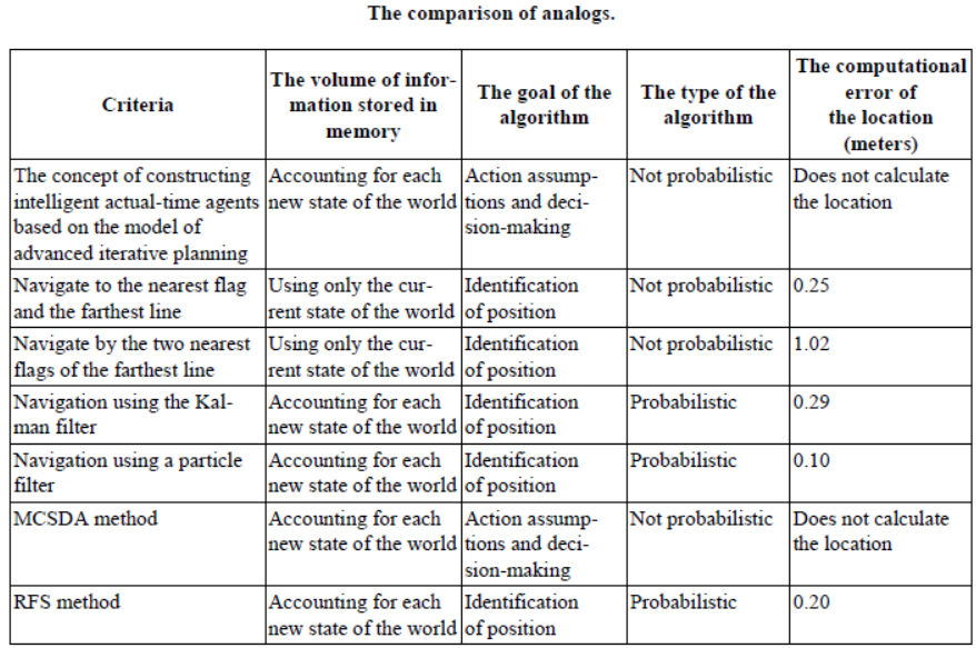
Methods that use only the operating cycle are faster than methods that use previous states of the world, but they have less ability to predict future states. The concept of constructing the intelligent actual-time agents based on the model of advanced iterative planning considers information starting from the first step of work, while it is possible to plan actions, and based on this, to predict the actions of agents, but the algorithm does not calculate coordinates. Navigation using the particle filter [13] demonstrates the highest calculation accuracy among all the presented algorithms, but at the same time the calculation takes the most time. The navigation methods using the Kalman filter, MCSDA, and RFC correspond to all the specified parameters, but their application depends on the problem and the available data.

The goal of this paper is to calculate the locations of objects, so the MCSDA algorithm will be excluded from consideration since it decides and navigates based on the already calculated locations of objects. The RFS method will be excluded from further consideration, since it is based on an obstacle map to get the location, and constructing this map for each player who has disappeared from consideration is an extremely resource-intensive problem.

Let's build a new algorithm for determining the coordinates of a player, including considering the prediction of the location of players who were recently per visual field, and then disappeared from it, based on the Kalman filter.

The Mathematical Model

Let's plan the problem as a mathematical model:

M = (I, P, C, F, O),

where I is the input data coming from the server. This data contains information about visible static (flags, lines, goals) and dynamic (ball, other players) objects in the field. I = {<f, l, g, b, a>}, where f is the set of received visible flags, l is the set of received visible lines, g is the set of visible goal flags, b is the set of ball positions consisting of a single element, and a is the set of visible agents.

P :I → C – the function of processing input data and calculating the coordinates of the agent, the coordinates of visible objects for the agent.

С = P(I) = {<k>} – calculation of coordinates for dynamic objects of a given game cycle, where k is the set of coordinates (x, y) for each dynamic object.

F :C → O – a data analysis function that performs a prediction using data about the current state of the world and the previous calculated states.

O = F(C) = {<k, p>} – the output data contains information about the location of visible objects for the current clock cycle and a forecast of actions for objects that have recently disappeared from the program's field of view.

k is the calculated coordinates for dynamic objects of the current game cycle, p is the action assumptions for objects that have disappeared from view, the assumption about the further movement of these objects.

Example of input data for the virtual soccer platform Soccer Simulation [3, 4]:

Flags (f) – reference objects placed in the field for calculating coordinates:

{

‘f b l 20 dist’: 43.8,

‘f b l 20 angle’: 10,

…}

Lines (l) – reference objects placed around the field for calculating coordinates:

{

‘l b dist’: 43.8,

‘f b l 20 angle’: -41,

…}

Gate (g) - reference objects placed in the field to identify different parts of the gate and calculate coordinates:

{

‘g r dist’: 100,

‘g r angle’: -44,

…}

The ball (b) is a dynamic object moving around the field. Based on the received information, it is possible to calculate the location of the ball:

{

‘b dist’: 33.1,

‘b angle’: 2,

…}

Visible players (a) - dynamic objects moving around the field. Based on the information received, it is possible to calculate the location of other players:

{

‘p "HELIOS2017" 2 dist’: 33.1,

‘p "HELIOS2017" 2 angle

’: -7,

…}

Figure 7 shows an example of an internal representation of the generated data based on the information received from the server.

Information about the player at number 1, where x and y are the calculated coordinates, absX and absY are the actual coordinates of the player, the angle is the orientation of the player in the field, speedX and speedY are the speed of the player at the corresponding coordinates (k is the calculated coordinates for the dynamic objects of the current game cycle):

x = -46.77

y = -5.88

absX = -47.49

absY = -5.12

angle = 2.28(radian)

speedX = 0.72

speedY = 0.44

Information about visible players 2 and 3, where viewPlayer is an array of names of visible players, mapPlayer contains a named array of visible players with a calculated location, while x, y are the calculated coordinates of the player, the angle is the orientation of the player on the field (k is the calculated coordinates for dynamic objects of the current game cycle):

otherPlayers.viewPlayer = ['b dist', 'p "HELIOS2017" 2', 'p "HELIOS2017" 3']

otherPlayers.mapPlayer = {

‘p "HELIOS2017" 2’: {

x: -27.53,

y: 3.18,

angle: -48

‘p "HELIOS2017" 3’: {

x: -28.51,

y: -1.77,

angle: -60

}

The action assumptions for objects that have disappeared from view (in this case, player 4), where x and y are the predicted coordinates, before and before are the calculated coordinates of the player in the previous step, the angle is the orientation of the player on the field, predictTick is the number of the predicted clock cycle (p is the forecast of actions for objects that have disappeared from view):

[{

‘p "HELIOS2017" 4’: {

x: -28.03,

y: 8.02,

beforeX: -27.53,

beforeY: 7.18,

angle: -51,

predictTick: 1

}

}]

Program Architecture

The structure of calculating the location of visible objects and constructing a forecast for objects that have disappeared from view includes the following sequence of actions:

- processing information about the current operating cycle to get the coordinates of visible dynamic objects;

- interaction with the state store to use information about previous operating cycles;

- predicting movement for dynamic * objects that have recently disappeared from view;

- saving information about the current state.

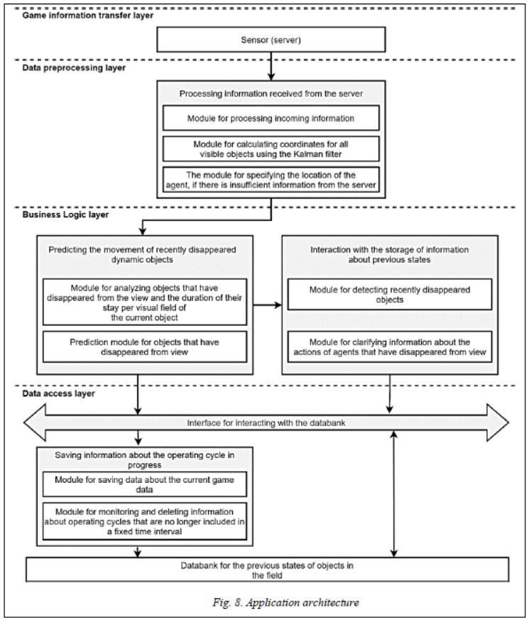
We can consider this sequence of actions as a basic set of architecture components (Fig. 8). Here, the components include specific modules:

- the processing component of the information received from the sensor receives and processes the information, as well as calculates the coordinates for all visible objects using the Kalman filter;

- the component of interaction with the storage of information about previous states performs the refinement of the agent's location when there is insufficient information from the server, the determination of objects that have recently disappeared from view, and the refinement of information about the actions of agents that have disappeared from view;

- the movement prediction component analyzes objects that have disappeared from view, the duration of their stay per visual field of the current object, and performs forecasting for objects that have disappeared from view;

- the component for saving information about the operating cycle saves data about the current game data and deletes information about clock cycles that are no longer included in a fixed time period.

Based on the model of the control program, we implement an algorithm for determining the coordinates of objects in the field using the Kalman filter and building an estimate for objects that have recently disappeared from view.

Step 1. Parsing and analyzing the information received from the server.

Step 2. If there are over two visible flags, then step 3, otherwise, the module for interaction with the information storage requests the last two states (operating cycles) and calculates the new location based on the coordinates, direction of movement, and speed. If the step is repeated for several bars of the game, then you must perform turns of the head or the complete body to get per visual field of at least two flags to clarify your location.

Step 3. The coordinates are calculated using the Kalman filter algorithm [13]. The correction is carried out according to the formulas:

x_i ₊₁ = x_i*K+(1 – K)*(x_i+ cos (α)*speedX),

y_i ₊₁ = y_i*K+(1 – K)*(y_i+ sin (α)*speedY),

where α is the direction of the player's body (in radians), speedX, speedY – the speed of movement along with the x and y coordinates, respectively.

Step 4. After determining the coordinates of the current player, the algorithm calculates the coordinates of the visible players by determining the coordinates of the three flags.

Step 5. Then the analysis of the players who disappeared from view and the duration of their stay per visual field of the current player is performed. If the player has been per visual field for two bars or more, then it is included in the set for which it performed the prediction.

Step 6. After receiving the array of analysis data, it predicted the new coordinates based on the last two states, from which the last known location, direction of movement, and speed of the object are determined.

Here are some examples of calculations.

1. After converting the input data, the information about the visible flags is an array of objects of the form:

[{

‘name’: ‘f b l 20 dist’

‘dist’: 43.8,

‘ angle’: 10,

}, …]

2. If the visible flags are less than two, then the basis for calculating the last two states is the calculation of the coordinates:

firstCoordVal.x = -9.01, firstCoordVal.y = 28.27

secondCoordVal.x = -8.42, secondCoordVal.y = 28.61

radian = 3.80

speedX = 0.59

speedY = -0.34

averageX = firstCoordVal.x + speedX * cos(radian) = -9.47

averageY = firstCoordVal.y + speedY * sin(radian) = 28.48

3. If there are over two visible flags, the coordinates of the two flags are calculated based on the received data about the flags:

[{

‘name’: ‘f b l 20 dist’

‘dist’: 43.8,

‘ angle’: 10,

}, …]

All possible pairs are cyclically iterated over, then the average for the corresponding coordinates is calculated:

averageX: -46.71, averageY: -6.64

4. Calculation of the error variance:

distanceMax = 111.0, distanceMix = 12.6

variance = ((distanceMax - distanceMix) ** 2) / 12 = ((111.0 – 12.6)^2)/12 = 806.88

5. Updating the Kalman coefficient:

varianceLast = 805.24

kalman = (varianceLast) / (varianceLast + variance) = 805.24/(805.24+806.88) = 0.4994

6. Correction using the Kalman coefficient:

speedX = 0.72, speedY = 0.44, radian = 2.29, coordLast.x = -46.36,

coordLast.y = -5.45

x = averageX * kalman + (1 - kalman) * (coordLast.x + speedX * cos(radian)) =

= -46.70 * 0.4994 + (1 - 0.4994) * (-46.35 + 0.72 * 2.29) = -46.77

y = averageY * kalman + (1 - kalman) * (coordLast.y + speedY *sin(radian)) =

= -6.64 * 0.4994 + (1 - 0.4994) * (-5.45 + 0.44 * 2.29) = -5.87

7. Next, we determine the coordinates of the visible players by three flags, the location of the current player always replaces one flag. Sample data:

‘p "HELIOS2017" 2 dist’: {

x: -27.53,

y: 3.18,

angle: -48

}

1. The analysis of the players who disappeared from view is performed, after which a list of objects that disappeared from view is obtained:

['p "HELIOS2017" 7 dist', 'p "HELIOS2017" 4 dist', 'p "Oxsy" 1 dist']

2. We perform the prediction after getting the last two states for the disappeared objects:

radian = 53.32

metPos[length-2].x = -25.63, metPos[length-2].y = -21.49

metPos[length-1].x = -27.34, metPos[length-1].y = -21.78

Based on this data, we get the object's speed:

speedX: 1.71, speedY: 0.29

Then the prediction:

predictX = metPos[length-1].x + speedX * cos(radian) = -27.34 + 1.71 * cos(53.32) =

= -29.05

predictY = metPos[length-1].y + speedY * sin(radian) = -21.78 +0.29 * sin(53.32) =

=-21.75

Experimental Results

For experimental research and comparative analysis of the proposed solution, they have developed a program in Python that implements the following functions:

- reading information about the game from the game protocol file and converting it to a format suitable for further work; the protocol file stores information about the actual state of the world for each operating cycle of the game and the data received by the players;

- calculation based on the transformed player location data;

- calculating the location of visible dynamic objects at the time point;

- analysis of objects that disappeared into the current operating cycle and prediction of their location;

- displaying the received data.

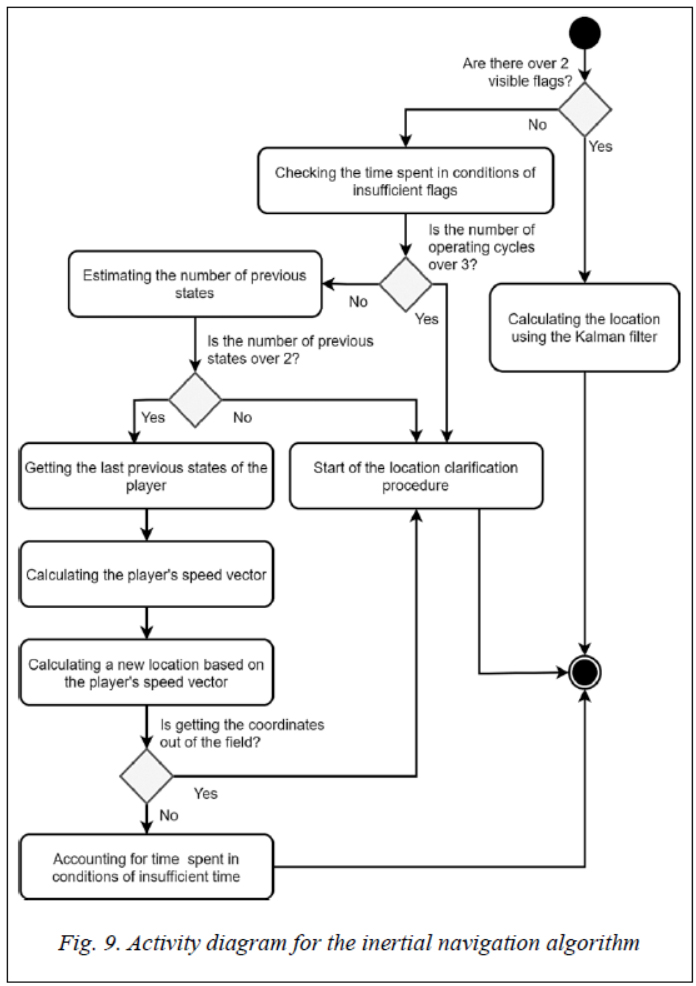
If there is enough information, i.e. there are over two visible flags, then the current player's location is determined using the Kalman filter [3, 14, 15]. In the conditions of insufficient flags, we use the algorithm for determining the location using the previous states according to the principle of inertial navigation (Fig. 9).

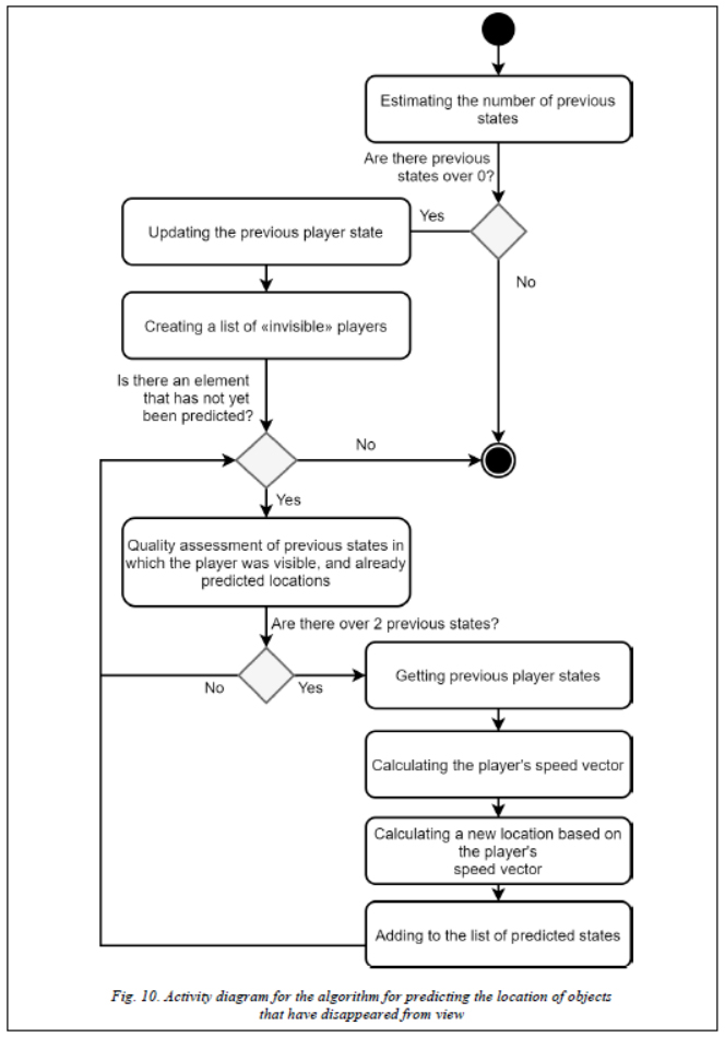
Forecasting comprises two stages:

- determining the list of disappeared objects;

- predicting the location of disappeared objects (Fig. 10).

Data for experiments are in [17]. In the middle of the experiments, it was found out that the proposed solution best predicts the location for objects located at a distance of two to five meters from the prediction start point, while the predictions can be considered valid for only ten cycles of the game (Fig. 11-14). The figures on the ordinate axis show the error of predicting new coordinates depending on the actual coordinates of the player (10, 12 – the average calculation error, 11, 13 – the calculation error standard deviation), on the abscissa axis are the numbers of the predicted clock cycles from the moment the player disappears from the field of view.

The error of predicting coordinates increases with the duration of the forecast, which is a consequence of the high dynamism of the game. For players moving at high speed, the quality of the forecast decreases. So, for objects those are over five meters from the beginning of the prediction point, the discrepancy in the accuracy of the prediction increases rapidly. This is because the average value of the player's movement for 10 cycles of the game varies from 1 to 4 m.

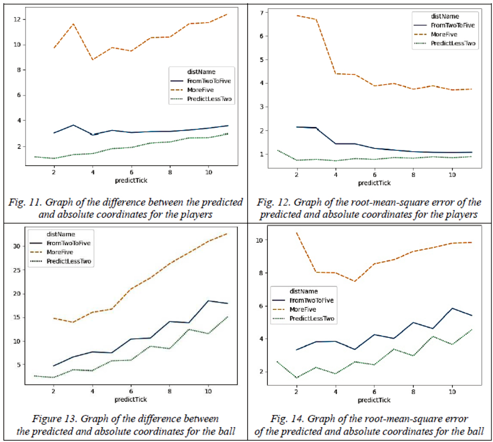
This case shows graphs for the game helios2017-vs-oxsy2017 from the storage, but similarly graphs were obtained for games between teams: oxsy2017-vs-hfutengine2017, oxsy2017-vs-helios2016.

Conclusion

The paper describes the solution to the problem of finding the location of virtual soccer players, including those who have disappeared from view. The last two known states of the player became the basis for forecasting. Based on the current position, the velocity vectors are also the basis for the forecast. The accuracy of the forecast is maximum when the player's position changes from 2 to 5 meters, at the minimum and maximum speeds, the average error increases rapidly. This is because the player's position changes from 2 to 5 meters. As a development, we proposed not only to model the coordinates of the player but also to analyze the situation in the field and predict the motives we perform for which this or that action. This may allow you to increase the accuracy of the forecast. We can use the developed program to analyze the situation in the field. In with decision-making systems, for example in [13], for processing incoming data. The next step is to check the operation of this system during the competition together with the decision-making systems.

References

1. Suzuki Y., Fukushima T., Thibout L., Nakashima T., Akiyama H. Game-Watching should be more entertaining: Real-time application of field-situation prediction to a soccer monitor. Proc. XXIII Intern. RoboCup Symposium, 2019, pp. 439–447. DOI: 10.1007/978-3-030-35699-6_35.

2. Visser A., Nardin L.G., Castro S. Integrating the latest artificial intelligence algorithms into the RoboCup rescue simulation framework. Proc. XXII Intern. RoboCup Symposium, 2019, pp. 476–487. DOI: 10.1007/978-3-030-27544-0_39.

3. Akiyama H., Nakashima T. (2014) HELIOS Base: An open source package for the RoboCup soccer 2D simulation. Proc. XVII Intern. RoboCup Symposium, 2014, pp. 528–535. DOI: 10.1007/978-3-662-44468-9_46.

4. Belyaev S.A. Mathematical Model of the Player Control in Soccer Simulation. Proc. 2021 ElConRus, 2021, pp. 233–237. DOI: 10.1109/ElConRus51938.2021.9396517.

5. Akiyama H., Nakashima T., Fukushima T., Zhong J., Suzuki Y., Ohori A. HELIOS2018: RoboCup 2018 soccer simulation 2D league champion. Proc. XXII Intern. RoboCup Symposium, 2019, pp. 450–461. DOI: 10.1007/978-3-030-27544-0_37.

6. Cano P., Ruiz-del-Solar J. Robust tracking of multiple soccer robots using random finite sets. Proc. XX Intern. RoboCup Symposium, 2017, pp. 206–217. DOI: 10.1007/978-3-319-68792-6_17.

7. Riccio F., Capobianco R., Nardi D. Using Monte Carlo search with data aggregation to improve robot soccer policies. Proc. XX Intern. RoboCup Symposium, 2017, pp. 256–267. DOI: 10.1007/978-3-319-68792-6_21.

8. Postnikov E.V., Belyaev S.A., Ekalo A.V., Shkulev A.A. Application of Fuzzy state machines to control players in virtual soccer simulation. Proc. EIConRus, 2019, pp. 291–294. DOI: 10.1109/EIConRus.2019.8657109.

9. Belyaev S.A. Application of probabilistic and time automata in control programs of multi-agent systems. H&ES Research, 2020, vol. 12, no. 3, pр. 47–53. DOI: 10.36724/2409-5419-2020-12-3-47-53 (in Russ.).

10. Pomas T., Nakashima T. Evaluation of situations in RoboCup 2D simulations using soccer field images. Proc. XXII Intern. RoboCup Symposium, 2019, pp. 275–286. DOI: 10.1007/978-3-030-27544-0_23.

11. Panteleev M.G. A conception of a real-time intelligent agents development on the basis of proactive iterative planning. Proc. XII National Conf. on Artificial Intelligence with International Participation KII-2012 , vol. 3, pp. 25–33 (in Russ.).

12. Belyaev S.A. Intellektualnye Sistemy. Programmirovanie Igrokov v Virtualnom Futbole . Saint Petersburg, 2020, 62 p. (in Russ.).

13. Panteleev M. G., Salimov A. F. Analysis of intelligent agent navigation algorithms in virtual football. Izvestiya SPbETU LETI, 2020, vol. 1, pp. 60–70 (in Russ.).

14. Dubrovin F.S., Shcherbatyuk A.F. Study of the algorithms for the single beacon mobile navigation of unmanned underwater vehicles: results of simulation and sea trials. Gyroscopy and Navigation, 2015, vol. 4, pp. 160–172. DOI: 10.17285/0869-7035.2015.23.4.160-172 (in Russ.).

15. Kucherskiy R.V., Man'ko S.V. Local navigation and mapping algorithms for the onboard control system of autonomous mobile robot. Izvestiya SFedU. Engineering Science, 2012, vol. 3, pp. 13–22 (in Russ.).

16. Chentsov D. A., Belyaev S.A. Monte Carlo tree search modification for computer games. Proc. EIConRus, 2020, pp. 252–255. DOI: 10.1109/EIConRus49466.2020.9039281.

17. RoboCupSimData Files Overview. Available at: http://oliver.obst.eu/data/RoboCupSimData/overview.html (accessed May 10, 2021).

УДК 004.421:004.832.24

DOI: 10.15827/2311-6749.21.2.1

Определение местонахождения игроков в виртуальном футболе

Д.А. Петруненко ¹ , студент, nokiad_1999@mail.ru

С.А. Беляев ¹ , к.т.н., доцент, bserge@bk.ru

¹ Санкт-Петербургский государственный электротехнический университет «ЛЭТИ» им. В.И. Ульянова (Ленина), Санкт-Петербург, 197376, Россия

Статья посвящена решению задачи определения местоположения игроков в виртуальном футболе. В качестве среды для проведения экспериментов использована платформа для проведения международных соревнований RoboCup 2D Soccer Simulation League. Информация о местоположениях объектов на поле является принципиально важной для принятия решения – необходимо определять местоположение игроков в условиях как полной, так и недостаточной информации. Использование предыдущих состояний и прогнозирование действий для недавно скрывшихся объектов позволяют улучшить точность прогноза развития ситуации на поле.

Авторы рассмотрели существующие решения по определению местоположения игроков и разработали новый алгоритм. При достаточности исходной информации для вычисления координат игрока используется фильтр Калмана, в условиях недостаточности информации – алгоритм инерциальной навигации, основанный на известных предыдущих состояниях.

В статье описан подход к прогнозированию местоположения игроков, которые недавно исчезли из поля зрения, рассмотрена математическая модель алгоритма, спроектирована архитектура программного решения. Разработанное решение проверено на нескольких реальных играх в среде виртуального футбола. Результаты представлены в виде графиков математического ожидания и дисперсии и подтверждают возможность прогнозирования местоположения недавно исчезнувших из виду объектов, вычислять координаты игрока в различных условиях.

С учетом полученных результатов определены направления дальнейших исследований по прогнозированию на основе не только предыдущих состояний, но и логики решений игроков. Следующий шаг – это интеграция разработанной программы в систему принятия решений для совместной проверки во время соревнований.

Ключевые слова: интеллектуальные агенты, виртуальный футбол, мультиагентные системы, позиционирование в условиях неопределённости, фильтр калмана, инерциальная навигация.

Литература

4. Belyaev S.A. Mathematical Model of the Player Control in Soccer Simulation. Proc. 2021 ElConRus, 2021, pp. 233–237. DOI: 10.1109/ElConRus51938.2021.9396517.

6. Cano P., Ruiz-del-Solar J. Robust tracking of multiple soccer robots using random finite sets. Proc.
XX Intern. RoboCup Symposium , 2017, pp. 206–217. DOI: 10.1007/978-3-319-68792-6_17.

9. Беляев С.А. Применение вероятностных и временных автоматов в программах управления многоагентных систем // Наукоемкие технологии в космических исследованиях Земли. 2020. Т. 12. № 3. С. 47–53. DOI: 10.36724/2409-5419-2020-12-3-47-53.

11. Пантелеев М.Г. Концепция построения интеллектуальных агентов реального времени на основе модели опережающего итеративного планирования // КИИ-2012: сб. тр. Белгород. 2012. Т. 3. С. 25–33.

12. Беляев С.А. Интеллектуальные системы. Программирование игроков в виртуальном футболе. СПб: Изд-во СПбГЭТУ «ЛЭТИ», 2020. 62 с.

13. Пантелеев М.Г., Салимов А.Ф. Анализ алгоритмов навигации интеллектуального агента в виртуальном футболе. Изв. СПбГЭТУ «ЛЭТИ». 2020. Т. 1. С. 60–70.

14. Дубровин Ф.С., Щербатюк А.Ф. Исследование некоторых алгоритмов одномаяковой мобильной навигации АНПА: результаты моделирования и морских испытаний // Гироскопия и навигация. 2015. Т. 4. С. 160–172. DOI: 10.17285/0869-7035.2015.23.4.160-172.

15. Кучерский Р.В., Манько С.В. Алгоритмы локальной навигации и картографии для бортовой системы управления автономного мобильного робота // Изв. ЮФУ: Технич. науки. 2012. Т. 3. С. 13–22.

16. Chentsov D. A., Belyaev S.A. Monte Carlo tree search modification for computer games. Proc. EIConRus, 2020, pp. 252–255. DOI: 10.1109/EIConRus49466.2020.9039281.

17. RoboCupSimData Files Overview. URL: http://oliver.obst.eu/data/RoboCupSimData/overview.html (дата обращения: 10.05.2021).

Литература

Comments